To investigate a new parameter identification or optimal control problem using PAREST we recommend to get a copy of all files of one of the examples and modify them for the new problem.
First, the file uspec.f of the problem dependent subroutines (described in Chapter 2) and the input file start.dat (described in Chapter 3) have to be prepared.
Next, the programs parest and pgraph can be compiled and linked by simply typing make (which makes use of the prepared Makefile).
parest The optimization is done by program parest. It is started by typing
parest
if the name of the input file is start.dat and the name of the output file is solution.dat. If input and/or output files do have other names they might be used as well. The syntax is
parest [-V i] [input file [output file]]
The terms in brackets ``[ ![]() ]'' may be supplied optionally
but don't have to be supplied always.
]'' may be supplied optionally
but don't have to be supplied always.
Using option -V i, the Verify Level i of NPSOL or NLSSOL may be set to either -1, 0, 1, 2, or 3 (cf. [9]). The default value is 0.
The default name of the output file is solution.dat. The output file contains a brief information about the optimization and two sections, namely STARTWERTE and STEUERUNG. These values can now be used as improved estimates of the state variables at the multiple shooting nodes (Section STARTWERTE of the input file) and of control variables at the control discretization grid points (Section STEUERUNG of the input file) for a subsequent run of PAREST if the corresponding sections of the input file are replaced by these values.
A run of PAREST can also be terminated interactively at any time by typing ;SPMlt;Ctrl;SPMgt;-c (or, of course, using the UNIX command kill on a UNIX machine). Then the program will respond by printing
Execution will be terminated
Please wait ...
The program will terminate immediately after the current
iteration has been completed and save the current estimate
of the solution in the output file solution.dat.
pgraph A graphical output is prepared by the post-processing program PGRAPH. It is based on the graphical system of the LRZ [3].
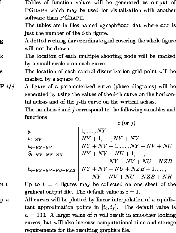
The program can be used with the following options

Description of options:


Curves corresponding to different runs of PAREST
can be drawn in the same figure by simply
listing the names of the corresponding output files
solution file ![]() ,..., solution file.
,..., solution file.
Also reference values from another source can be drawn in the same figure as the solution of PAREST. They have to be provided in form of tables of function values. These files have to be distinguished from solutions files of PAREST by typing "`#"' as an initial to their file names.
The format of such tables with reference values is:
number of function values number of functions
curve number
![]()
![]() curve number
curve number ![]()

The numbers of curves are interpreted in a way described for option -P. If one of the columns of the table may not be drawn then the curve number -1 has to be used.
User defined functions of the state and control variables may also be plotted. This is done by defining them as additional functions appended to the measurement functions h.
Examples for calls of PGRAPH:
For example, consider a problem with the dimensions NY = DIMY = 2, NV = DIMV = 0, NU = DIMU = 0, NZB = 1, NH = DIMH = 1.
The first two rows of the file with 100 reference values for 5 variables or functions in tables to be drawn in comparison with the solutions of PAREST may read as
100 5
0 1 3 -1 2 4
Now the interpretation of the columns of the tabular values which are following these two rows is
![]()
As standard output, pgraph generates an output file named ZZZG67 which is prepared for previewing by the command graphik of [3].
Examples for calls of graphik:
Refinement of the control functions
The function tables generated by the -l option of
PGRAPH can be used to obtain a finer approximation of
the control variables u.
For example we have a solution of an optimization problem where the control
function has been calculated at 10 equidistant points. In
the next optimization run we like to refine the control and
calculate its values at 20 equidistant points. The following
run of PGRAPH generates a function table of all variables
in the file pgraph#00.gdat at the desired locations:
pgraph -l -p 20 solution.dat
Assume we have three state variables and one control function, then the function table contains five columns. The first column holds the time, the following three the corresponding values of the state variables and the fifth the values of the control variable.
The following awk script extracts the values of the control function out of the file pgraph#00.gdat and prints a new section for the control:
BEGIN   { print "STEUERUNG" }

/^[^#]/ { # Each line not beginning with '#'
          print "   T =   ", $1
          print "      U(1) = ", $5
        }

END     { print "ENDE" }
If we name the script genu.awk the new section is generated by
typing
awk -f genu.awk < 'pgraph#00.gdat' > newu.dat
Finally we have to replace the section STEUERUNG in the file
solution.dat by the new one in newu.dat. We now can
invoke the optimization with
parest start.dat solution.dat