This problem describes the lifting of
an airbreathing lower stage of a two-stage-to-orbit
Sänger-type launch vehicle. We focus on the Ramjet-powered
second part of the trajectory.
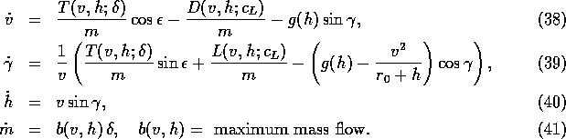
The four state variables are the velocity v, the flight path angle  ,
the altitude h, and the mass m. The three control variables
are the lift coefficient
,
the altitude h, and the mass m. The three control variables
are the lift coefficient  , the thrust angle
  and the
throttle setting
and the
throttle setting  ,
,  .
The equations of motion are
.
The equations of motion are
The considered time interval is  and
and  is free.
The following formulae are used for the thrust, the lift and the
drag forces
is free.
The following formulae are used for the thrust, the lift and the
drag forces
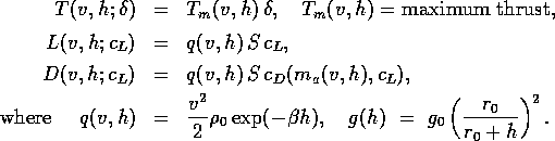
The lift and drag model has a quadratic polar
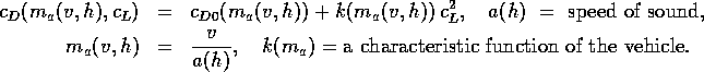
The quantities  , and
, and  are constants.
For more details of the problem and for a three dimensional formulation
cf. Chudej [7].
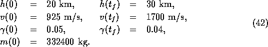
The boundary conditions are
are constants.
For more details of the problem and for a three dimensional formulation
cf. Chudej [7].
The boundary conditions are
The objective is to maximize the final mass, i. e.,

Here, the direct collocation method was applied on a rather bad initial estimate
of the optimal trajectory. For the states, the boundary values have been
interpolated linearly and the controls have been set to zero.
The direct collocation method DIRCOL
converges in two macro
iteration steps to a solution with 21 grid points.
From this solution, the optimal states and the
adjoint variables have been estimated.
Based on this estimate, the multiple shooting method was applied
to solve the boundary value problem arising from
the optimality conditions (see [7]).
The final solutions are 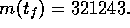 kg and
  s.
For these values, the solution of the direct collocation method
was accurate to four digits.
s.
For these values, the solution of the direct collocation method
was accurate to four digits.
In Figs. 1 to 6, the solution of the direct collocation method is
shown by a dashed line and the highly accurate solution of the multiple shooting method
is shown by a solid line.
In the figures, there is no visible difference between the
suboptimal and the optimal state variables.
Also, the estimated adjoint variables and the suboptimal controls of the
direct collocation method show a pretty good conformity with the highly accurate ones.
The approximation quality can furthermore be improved
by increasing the number of
grid points to more than 21.
The optimal throttle setting  equals one
within the whole time interval as it is found by both methods.
equals one
within the whole time interval as it is found by both methods.
=5.2cm =7.3cm ZZZG67_altitude.epsf
=5.2cm =7.3cm ZZZG67_fl_p_angle.epsf
Fig. 1: The altitude  .
Fig. 2: The flight path angle
.
Fig. 2: The flight path angle  .
.

*[-3.0cm]
=5.2cm =7.3cm ZZZG67_lambda_altitude.epsf
=5.2cm =7.3cm ZZZG67_lambda_fl_p_angle.epsf
*[0.3cm]
Fig. 3: The adjoint variable  .
Fig. 4: The adjoint variable
.
Fig. 4: The adjoint variable  .
.
*[-1.6cm]
=5.2cm =7.3cm ZZZG67_lift_coef.epsf
=5.2cm =7.3cm ZZZG67_thrust_angle.epsf
*[0.3cm]
Fig. 5: The lift coefficient  .
Fig. 6: The thrust angle
.
Fig. 6: The thrust angle  .
.